Hans-Juergen Schoenig: Using “Row Level Security” to make large companies more secure

2019-09-28

Hans-Juergen Schoenig: Using “Row Level Security” to make large companies more secure

https://postgr.es/p/4A9

Large companies and professional business have to make sure that data is kept secure. It is necessary to defend against internal, as well as external threats. PostgreSQL provides all the necessities a company needs to protect data and to ensure that people can only access what they are supposed to see. One way to protect data is “Row Level Security”, which has been around for some years now. It can be used to reduce the scope of a user by removing rows from the result set automatically. Usually people apply simple policies to do that. But, PostgreSQL Row Level Security (RLS) can do a lot more. You can actually control the way RLS behaves using configuration tables.

Configuring access restrictions dynamically

Imagine you are working for a large cooperation. Your organization might change, people might move from one department to the other or your new people might join up as we speak. What you want is that your security policy always reflects the way your company really is. Let us take a look at a simple example:

CREATE TABLE t_company
(
     id            serial,
     department    text NOT NULL,
     manager       text NOT NULL
);

CREATE TABLE t_manager
(
     id      serial,
     person  text,
     manager text,
     UNIQUE (person, manager)
);

I have created two tables. One will know, who is managing which department. The second table knows, who will report to him. The goal is to come up with a security policy, which ensures that somebody can only see own data or data from departments on lower levels. In many cases row level policies are hardcoded – in our case we want to be flexible and configure visibility given the data in the tables.

Let us populate the tables:

INSERT INTO t_manager (person, manager)
VALUES ('hans', NULL),
       ('paula', 'hans'),
       ('berta', 'hans'),
       ('manuel', 'paula'),
       ('mike', 'paula'),
       ('joe', 'berta'),
       ('jack', 'berta'),
       ('jane', 'berta')
;

hierarchy


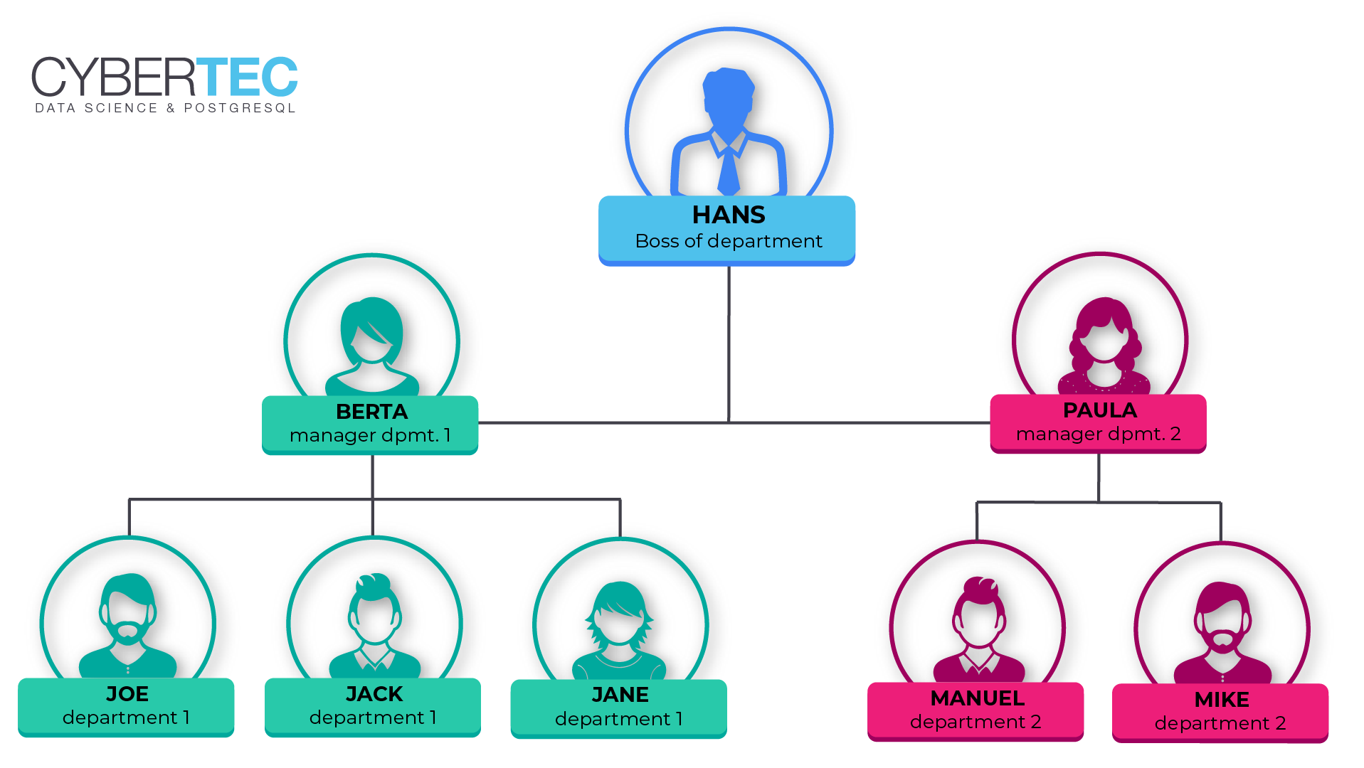
As you can see “hans” has no manager. “paula” will report directly to “hans”. “manuel” will report to “paula” and so on.

In the next step we can populate the company table:

INSERT INTO t_company (department, manager)
VALUES ('dep_1_1', 'joe'),
       ('dep_1_2', 'jane'),
       ('dep_1_3', 'jack'),
       ('dep_2_1', 'mike'),
       ('dep_2_2', 'manuel'),
       ('dep_1', 'berta'),
       ('dep_2', 'paula'),
       ('dep', 'hans')
;

For the sake of simplicity, I have named those departments in a way that they reflect the hierarchy in the company. The idea is to make the results easier to read and easier to understand. Of course, any other name will work just fine as well.

Defining row level policies in PostgreSQL

To enable row level security (RLS) you have to run ALTER TABLE … ENABLE ROW LEVEL SECURITY:

ALTER TABLE t_company ENABLE ROW LEVEL SECURITY;

What is going to happen is that all non-superusers, or users who are marked as BYPASSRLS, won’t see any data anymore. By default, PostgreSQL is restrictive and you have to define a policy to configure the desired scope of users. The following policy uses a subselect to travers our organization:


CREATE POLICY my_fancy_policy
  ON t_company
  USING (manager IN ( WITH RECURSIVE t AS 
                        (
                           SELECT current_user AS person, NULL::text AS manager
                           FROM t_manager
                           WHERE manager = CURRENT_USER
                           UNION ALL
                           SELECT m.person, m.manager
                           FROM t_manager m
                           INNER JOIN t ON t.person = m.manager
                        )
                        SELECT person FROM t
                    )
        )
;

What you can see here is that a policy can be pretty sophisticated. It is not just a simple expression but can even be a more complex subselect, which uses some configuration tables to decide on what to do.

PostgreSQL row level security in action

Let us create a role now:

CREATE ROLE paula LOGIN;
GRANT ALL ON t_company TO paula;
GRANT ALL ON t_manager TO paula;

paula is allowed to log in and read all data in t_company and t_manager. Being able to read the table in the first place is a hard requirement to make PostgreSQL even consider your row level policy.

Once this is done, we can set the role to paula and see what happens:

test=> SET ROLE paula;
SET
test=>; SELECT * FROM t_company;

id  | department | manager
----+------------+---------
4   | dep_2_1    | mike
5   | dep_2_2    | manuel
7   | dep_2      | paula
(3 rows)

As you can see paula is only able to see herself and the people in her department, which is exactly what we wanted to achieve.

Let us switch back to superuser now:

SET ROLE postgres;

We can try the same thing with a second user and we will again achieve the desired results:


CREATE ROLE hans LOGIN;

GRANT ALL ON t_company TO hans;
GRANT ALL ON t_manager TO hans;

The output is as expected:

test=# SET role hans;
SET
test=> SELECT * FROM t_company;
id  | department | manager
----+------------+---------
1   | dep_1_1    | joe
2   | dep_1_2    | jane
3   | dep_1_3    | jack
4   | dep_2_1    | mike
5   | dep_2_2    | manuel
6   | dep_1      | berta
7   | dep_2      | paula
8   | dep        | hans
(8 rows)

Row level security and performance

Keep in mind that a policy is basically a mandatory WHERE clause which is added to every query to ensure that the scope of a user is limited to the desired subset of data. The more expensive the policy is, the more impact it will have on performance. It is therefore highly recommended to think twice and to make sure that your policies are reasonably efficient to maintain good database performance.

The performance impact of row level security in PostgreSQL (or any other SQL database) cannot easily be quantified because it depends on too many factors. However, keep in mind – there is no such thing as a free lunch.

If you want to learn more about Row Level Security check out my post about PostgreSQL security.

The post Using “Row Level Security” to make large companies more secure appeared first on Cybertec.

postgresql

via Planet PostgreSQL https://ift.tt/2g0pqKY

September 24, 2019 at 09:43AM

Enrico Zini: xtypeinto: type text into X windows

2019-09-25

Enrico Zini: xtypeinto: type text into X windows

https://ift.tt/2mwzljt

Several sites have started disabling paste in input fields, mostly password
fields, but also other fields for no apparent reason.

Random links on the topic:

This said, I am normally uneasy about copy-pasting passwords, as any X window
can sniff the clipboard contents at any time, and I like password managers like
impass that would type it for you
instead of copying it to the clipboard.

However, today I got out way more frustrated than I could handle after illing
in 17-digits nonsensical, always-slightly-different
INPS
payment codelines inside input fields that disabled paste for no reason
whatsoever (they are not secret).

I thought "never again", I put together some code from
impass and
wmctrl and created
xtypeinto:

$ ./xtypeinto --help
usage: xtypeinto [-h] [--verbose] [--debug] [string]

Type text into a window

positional arguments:
  string         string to type (default: stdin)

optional arguments:
  -h, --help     show this help message and exit
  --verbose, -v  verbose output
  --debug        debug output

Pass a string to xtypeinto as an argument, or as standard input.

xtypeinto will show a crosshair to pick a window, and the text will be typed
into that window.

Please make sure that you focus on the right field before running xtypeinto,
to make sure things are typed where you need them.

via Planet Debian https://ift.tt/2hZnWDQ

September 24, 2019 at 04:06PM

Enrico Zini: Upgrading LineageOS 14 to 16

2019-09-23

Enrico Zini: Upgrading LineageOS 14 to 16

https://ift.tt/30ixO3f

The LineageOS updater notified me that there will be no more updates for
LineageOS 14, because now development on my phone happens on LineageOS 16,
so I set aside some time and carefully followed the upgrade instructions.

I now have a phone with Lineageos 16, but the whole modem subsystem does not
work.

Advice on #lineageos was that "the wiki instructions are often a bit generic..
offical thread often has the specific details".

Official thread is
here,
and the missing specific detail was "Make sure you had Samsung’s Oreo firmware
bootloader and modem before installing this.".

It looks like nothing ever installed firmware updates, since the Android that
came with my phone ages ago. I can either wipe everything and install a stock
android to let it do the upgrade, then replace it with LineageOS, or try a
firmware upgrade.

This link
has instructions for firmware upgrades using haimdall, which is in Debian,
instead of Odin, which is in Windows.

Finding firmwares is embarassing. They only seem to be available from links on
shady download sites, or commercial sites run by who knows whom. I verify
sha256sums on LineageOS images, F-Droid has reproducible builds, but at the
base of this wonderful stack there’s going to be a blob downloaded off some
forum on the internet.

In this case, this link points to some collection of firmware blobs.

I downloaded the pack and identified the ones for my phone, then unpacked the
tar files and uncompressed the lz4 blobs.

With heimdall, I identified the mapping from partition names to blob names:

heimdall print-pit --no-reboot

Then I did the flashing:

heimdall flash --resume --RADIO modem.bin --CM cm.bin --PARAM param.bin --BOOTLOADER sboot.bin

The first time flashing didn’t work, and I got stuck in download mode.
This
explains how to get out of download mode (power + volume down for 10s).

Second attempt worked fine, and now I have a working phone again:

heimdall flash --RADIO modem.bin --CM cm.bin --PARAM param.bin --BOOTLOADER sboot.bin

via Planet Debian https://ift.tt/2hZnWDQ

September 20, 2019 at 05:23PM

Kaarel Moppel: A Primer on PostgreSQL Upgrade Methods

2019-09-09

Kaarel Moppel: A Primer on PostgreSQL Upgrade Methods

https://postgr.es/p/4zy

Soon it’s that time of the year again – basically a 2nd Christmas for followers of the “blue elephant cult” if you will :). I’m, of course, referring to the upcoming release of the next PostgreSQL major version, v12. So I thought it’s about time to go over some basics on upgrading to newer major versions! Database upgrades (not only Postgres) are quite a rare event for most people (at least for those running only a couple of DB-s). Since upgrades are so rare, it’s quite easy to forget how easy upgrading actually is. Yes, it is easy – so easy that I can barely wrap my head around why a lot of people still run some very old versions. Hopefully, this piece will help to convince you to upgrade faster in the future :). For the TLDR; (in table version) please scroll to the bottom of the article.

Why should I upgrade in the first place?

Some main points that come to my mind:

  • More security
    Needless to say, I think security is massively important nowadays! Due to various government regulations and the threat of being sued over data leaks, mistakes often carry a hefty price tag. Both new and modern authentication methods and SSL/TLS version support are regularly added to new PostgreSQL versions.
  • More performance without changing anything on the application level!
    Based on my gut feeling and on some previous testing, typically in total around ~5-15% of runtime improvements can be observed following an upgrade (if not IO-bound). So not too much…but on some releases (9.6 parallel query, 10.0 JIT for example) a possibly game changing 30-40% could be observed. As a rule, the upgrades only resulted in upsides – over the last 8 years, I’ve only seen a single case where the new optimizer chose a different plan so that things got slower for a particular query, and it needed to be re-written.
  • New features for developers
  • Every year, new SQL standard implementations, non-standard feature additions, functions and constructs for developers are introduced, in order to reduce the amounts of code written – or to achieve something that was very hard, or possible only on the application layer.
  • Better DBA / management features
    Better high-availability, backup, monitoring and scaling features for DBA-s.  The last couple of releases have been a real boon in these matters for example with Logical Replication, partitioning and built-in monitoring roles.

And to make it even more easy for you – there’s a really cool website (much kudos to Depesz!) where you can directly get a highlighted listing of all the changes between two target Postgres versions! Link here!


Minor Updates

Minor version changes a.k.a. bugfix releases happen  regularly and can be used as a warmp-up (there is a minimum of 1 release per quarter, if no security-critical stuff is found). Itt is, of course, highly recommended to apply them as soon as they are released.

The good thing about minor releases is that they’re as fast as restarting your server! I recommend to “prefix” the restart  with a hand-initiated “checkpoint” so that effective downtime for applications is minimized since “pg_ctl stop / restart” already does checkpointing in exclusive mode, after active sessions have been kicked from the server.

Caution! When using some distribution-specific Postgres packages some extra attention is needed. For example running “apt upgrade postgresql-X” might mean an imminent restart to the running instance, after new binaries have been pulled in! For RedHat / CentOS it’s usually a bit better though and there you need to restart explicitly.

Also when running a clustered (streaming replication) setup where downtime on the primary node is scarce and restarts are to be avoided, my recommendation is to immediately update all replicas to the latest minor version (minor versions don’t need to match). That way, when some accidental server issue appears (i.e. reboot, hardware maintenance etc) you’ll already be promoted to the latest version with a sort of “free downtime”.

Let’s now move on to the real thing – major upgrade options.


Logical Dump / Restore

This is the original way of doing major version upgrades and it’s the only option up until version 9.0 which introduced the binary / in-place option. Logical dumps use “pg_dumpall” or “pg_dump” / “pg_restore” tools, that basically “reverse engineer” the database state to normal SQL statements. When those statements are executed sequentially on a target DB, they re-create exactly the same state for all user-level objects as it was on the source cluster / DB. NB! “Pg_dumpall” works on the instance level and “pg_dump” on the database level.

PROS:

  • 100% safe – the original instance is not changed in any way so testing etc is quite easy and straightforward and rolling back is also no problem.
  • Dumps can theoretically be pulled online or from a degraded “read only” instance. The only thing to watch out for: make sure your applications are stopped (or access limited on Postgres side) when pulling the “dump”, as it will only contain a snapshot of the data from the exact moment when the process was launched. If any rows are changed after that, they will be lost if they have not been picked up by some 3rd party “merge” tools (like dbForge for example).
  • Flexible – there are lots of flags to only dump / restore specific objects or schemas, re-map or remove ownership / access privileges. Data can also be represented with SQL standard INSERT statements so theoretically one could also move between different database systems.

CONS:

  • Slow – although pg_dump / pg_restore on modern PG versions can be parallelized very easily for better performance longer downtimes might be unavoidable. In practice you start to notice problems around 100GB, especially when you have a lot of indexes and constraints. This is where most of the time will be typically burnt during restore as it’s both CPU and disk intensive.
  • Possibly a “per database” approach is needed, where consistency on the instance level is not guaranteed out of the box (see“pg_dump –snapshot” param for a workaround).

One more recommendation – when dumping out the DB contents it’s usually best to use the tools from the latest Postgres version. Note that this might not be officially supported, if you fall out of the “5 latest releases supported” window. By the way, on the topic of dump / restore and Postgres versions, I’d recommend to read this nice FAQ by our colleague Pavlo. It’s a few years old, but still correct.


Binary In-Place Upgrades

Binary in-place upgrades are quite different from the logical ones as they happen on the filesystem level (i.e. always on the same machine if no shared storage is in play) and are a multi-step process with some additional complexity. However, things are still quite straightforward – after installing the new binaries and following a bit of preparation, it basically boils down to running a single command that typically finishes in 10 to 20 seconds in “–link” mode!! That’s also why it’s the most common upgrade option nowadays: nobody wants extended downtimes.

High-level steps to take (see documentation for details):

1. Install new major version binaries.
2. Initialize the new instance with new binaries (with the same major settings as on the old instance).
3. Do a test run with “pg_upgrade”. FYI – I tend to test first on a completely spare replica or a P.I.T.R. restored instance.
4. Stop the old instance.
5. Run “pg_upgrade” with or without file linking. Using hard-linking of files from the old data directory into the new one is the fastest way to upgrade! Basically only system catalogs are dumped and reloaded. Without linking all data files are copied over and it boils down to filesystem speed vs instance size, with the benefit that the old cluster is not modified.
6. Start the instance (it is usually also necessary to change the port back to 5432).
7. Start the “analyze” script generated and hinted at by the “pg_upgrade” tool. Performance for complex queries might suffer until it finishes.

PROS:

  • Typically very fast. Especially with “pg_upgrade –link –jobs X”.

CONS:

  • More risky: more things can theoretically go wrong (especially in “–link” mode), so some extra testing would be nice. At a minimu, after performing a successful upgrade process (for more important DB-s) I do a quick logical dump / restore (heavily parallel if possible) on the side. If that would take too long for large instances I at least make sure that a dump to /dev/null runs through clean. For large instances, I also tend to utilize some homw-brewed scripts to dump single tables independently. Doing that avoids the negative effects of a prolonged snapshot. It only makes sense to do so as long as the DB is not a humongous single table (which we see far more often than we should).
  • All extensions and other modules also need to be present for the new version – this could be especially burdensome if using a lot of 3rd party extensions
  • No semi-online mode – always real downtime incurred, albeit short.
  • You lose all standby servers if not using “–link” mode! With “–link” there are some ways to get around that problem though if an extended downtime allows it – see here for details.
  • Degraded 1st startup. The upgrade process currently does not copy over any statistics on our data distributions! This is stuff like histogram, most common values and their frequencies and could mean a considerable performance hit for complex queries before our “vacuumdb –analyze-only –analyze-in-stages” finishes.

NB! Also note that some distributions provide wrapper scripts (like “pg_upgradecluster” on Debian-based systems) to assist with in-place upgrades. They might be worth a look.

Logical Replication

Logical Replication (LR) is the latest addition to the family of Postgres major version upgrade options and is available from v10 and upwards. By the way, unofficially it’s also already possible from 9.4 and upwards so feel free to contact us on that if you can’t afford extended downtime for your older instances. But OK, how does this new thing work? Some sample code is well demonstrated here, so I won’t go into technical details myself.  In general, it works on the DB level: you’re going to be feeding all old data and data changes from the old primary into a newly bootstrapped and schema-synchronized fully independent master / primary server! Basically LR is about decoupling from the binary “on-disk” format and sending over data objects that could be thought of as kind of JSON. Again, to highlight the major benefit here: the servers are for the most part fully decoupled and the syncing process happens in near realtime, so one can take some time to test and validate the results before flipping the final switch!

It looks awesome and relatively simple, doesn’t it? And it is mostly! To spoil the party a bit – there’s also a lot of “small print” to read, and an out-of-the box LR process might not always be possible – it depends a bit on the data model being used. Some tweaking / changing might be needed.

PROS:

  • Flexible. One can for example already make some changes on the target DB – new columns, indexes etc…
  • Safe. One should only watch out for the replication slot on the source DB if the process is canceled or the target server taken down suddenly.
  • Minimal downtime required.

CONS:

  • Quite a few steps to take.
  • Could take a long time for big databases.
  • Possibly there will be a need to modify the schema or at least REPLICA IDENTITY.


Summary of Pros / Cons for Different Upgrade Methods

Upgrade method Pro Contra
Dump / restore
  • Simple
  • Safe
  • Somewhat flexible
  • Slowest method
  • Per database approach has some pitfalls lurking
Binary in-place
  • Fast / very fast (depending on chosen mode)
  • Old instance not affected in default mode
  • More complex than Dump / Restore
  • Somewhat risky in “link” mode
  • Possibly loses standby servers
  • Double the disk space required in default mode
Logical Replication
  • Shortest possible downtime
  • Safe, with possibility of thorough “live tests”
  • Very flexible
  • Most complex method
  • Possibly some schema changes needed
  • Possibly “slowish”
  • Always per database

Some General Advice and Parting Words

I guess besides the obvious pre-upgrade DBA activities (testing, backups, thoroughly analyzing the release notes) for all upgrade methods, it’s also good to discuss some other things like application compatibility and UI or monitoring tools compatibility with end users / application teams. But truth be told – there is actually a very low risk factor involved in upgrading, main SQL features are backwards compatible.

I can’t of course 100% recommend doing “lone ranger” types of covert database migrations (although I’ve done my fair share of these) where the DB disappears for a minute to then reappear in a shiny new “coat” without anyone raising an eyebrow. However, if your schema consists only of a handful of plain tables with the most common data types (no stored procedures or other PostgreSQL specific features like LISTEN / NOTIFY) and standard ANSI SQL is performed then most likely everything will be just fine. This is due to the fact that the Postgres wire protocol has not been changed since v7-point-something. Changing it for basic SQL operations would be a massive problem for all users globally. That’s why changing it has been avoided.

If you’re not running an absolutely time-critical 24/7 operation (something like a space-shuttle) in my opinion there are no excuses not to upgrade at least once every couple of years. Keep in mind – if you ignore the topic for too long you’ll stop receiving security patches at some point. Then, when it is most needed, the upgrade process becomes slightly more tricky, since the PostgreSQL Global Development Group only supports releases from the previous 5 years in it’s tooling. If you’ve waited too long, you might need to run “pg_upgrade” twice in a row and there’s some additional risk of stumbling into some cornercase backwards compatibility topics, as there’s no testing for such scenarios. In short, upgrade – sooner better than later!

The post A Primer on PostgreSQL Upgrade Methods appeared first on Cybertec.

postgresql

via Planet PostgreSQL https://ift.tt/2g0pqKY

September 7, 2019 at 11:46AM

Hans-Juergen Schoenig: PostgreSQL: Trivial timeseries examples

2019-08-24

Hans-Juergen Schoenig: PostgreSQL: Trivial timeseries examples

https://postgr.es/p/4yq

Timeseries are an increasingly important topic – not just in PostgreSQL. Recently I gave a presentation @AGIT in Salzburg about timeseries and I demonstrated some super simple examples. The presentation was well received so I decided to share this stuff in the form of a blog PostgreSQL, so that more people can learn about windowing functions and SQL in general. A link to the video is available at the end of the post so that you can listen to the original material in German.

Loading timeseries data the easy way

To show how data can be loaded, I compiled a simple dataset, which can be found on my website. Here is how it works:

test=# CREATE TABLE t_oil 
(
	region 		text, 
	country 	text, 
	year 		int, 
	production 	int, 
	consumption 	int
);
CREATE TABLE
test=# COPY t_oil FROM 
	PROGRAM 'curl https://www.cybertec-postgresql.com/secret/oil_ext.txt';
COPY 644

The cool thing is that if you happen to be a superuser you can easily load the data from the web directly. COPY FROM PROGRAM allows you to execute code on the server and pipe it directly to PostgreSQL, which is super simple. But keep in mind: This only works if you are a PostgreSQL superuser (for security reasons).

lag: The backbone of timeseries analysis

If you are dealing with timeseries calculating the difference to the previous period is really important and is needed in many cases. Fortunately SQL allows you to do that pretty easily. Here is how it works:

test=# SELECT year, production, 
		lag(production, 1) OVER (ORDER BY year) 
	FROM 	t_oil 
	WHERE 	country = 'USA' 
	LIMIT 5;
 year | production |  lag  
------+------------+-------
 1965 |       9014 |      
 1966 |       9579 |  9014
 1967 |      10219 |  9579
 1968 |      10600 | 10219
 1969 |      10828 | 10600
(5 rows)

The lag functions takes two parameters: The first column defines the column, which should be used in this case. The second parameter is optional. If you skip it the expression will be equivalent to lag(production, 1). In my example the lag column will be off by one. However, you can use any integer number to move data up or down given the order defined in the OVER clause.

What we got so far is the value of the previous period. Let us calculate the difference next:

test=# SELECT year, production, 
		production - lag(production, 1) OVER (ORDER BY year) AS diff 
	FROM 	t_oil 
	WHERE 	country = 'USA' 
	LIMIT 5;
 year | production | diff 
------+------------+------
 1965 |       9014 |     
 1966 |       9579 |  565
 1967 |      10219 |  640
 1968 |      10600 |  381
 1969 |      10828 |  228
(5 rows)

That was easy. All we have to do is to take the current row and subtract the previous row.
Windowing functions are ways more powerful than shown here but maybe this example is good to getting you started in the first place.

Calculating correlations using PostgreSQL

Sometimes you might want to calculate the correlation between columns. PostgreSQL offers the “corr” function to do exactly that. The following listing shows a simple example:

test=# SELECT country, corr(production, consumption) 
	FROM 	t_oil 
	GROUP BY 1 
	ORDER BY 2 DESC NULLS LAST;
       country        |        corr        
----------------------+--------------------
 Mexico               |  0.962790640608018
 Canada               |  0.932931452462893
 Qatar                |  0.925552359601189
 United Arab Emirates |  0.882953285119214
 Saudi Arabien        |  0.642815458284221

As you can see the correlation in Mexico and Canada are highest.

Checking for continuous activity

In the past we presented other examples related to timeseries and analysis in general. One of the most interesting posts is found here.

If you want to see the entire short presentation in German consider checking out the following video.

The post PostgreSQL: Trivial timeseries examples appeared first on Cybertec.

PostgreSQL

postgresql

via Planet PostgreSQL https://ift.tt/2g0pqKY

August 13, 2019 at 11:58AM

Add A Microscope To Your 3D Printer

2019-08-13

Add A Microscope To Your 3D Printer

https://ift.tt/2YDAJSx

There are many ways to keep an eye on your 3D printer as it churns out the layers of your print. Most of us take a peek every now and then to ensure we’re not making plastic vermicelli, and some of us will go further with a Raspberry Pi camera or similar. [Uri Shaked] has taken this a step further, by adding a USB microscope on a custom bracket next to the hot end of his Creality Ender 3.

The bracket is not in itself anything other than a run-of-the-mill piece of 3D printing, but the interest comes in what can be done with it. The Ender 3 has a resolution of 12.5μm on X/Y axes, and 2.5μm on Z axes, meaning that the ‘scope can be positioned to within a hair’s-breadth of any minute object. Of course this achieves the primary aim of examining the integrity of 3D prints, but it also allows any object to be tracked or scanned with the microscope.

For example while examining a basil leaf, [Uri] noticed a tiny insect on its surface and was able to follow it with some hastily entered G-code. Better still, he took a video of the chase, which you can see below the break. From automated PCB quality control to artistic endeavours, we’re absolutely fascinated by the possibilities of a low-cost robotic microscope platform.

[Uri] is a perennial among Hackaday-featured projects, and has produced some excellent work over the years. Most recently we followed him through the production of an event badge.

hardware

via Hack a Day https://hackaday.com

August 4, 2019 at 04:07AM

Tatsuo Ishii: Automatically updating materialized views

2019-08-07

Tatsuo Ishii: Automatically updating materialized views

https://postgr.es/p/4yc

Materialized views are convenient and efficient way to retrieve information from database. Unlike ordinary views, materialized views save the query result and provide faster access to the data. For example, user can create a simple materialized view containing the number of rows in a table:

 CREATE MATERIALIZED VIEW mv1 AS SELECT count(*) FROM pgbench_accounts;

Obtaining the number of rows using the materialized view mv1 is much faster than  directly accessing number of rows in pgbench_accounts.

test=# SELECT * from v1;
 count 
——–
 100000
(1 row)

Time: 0.810 ms
test=# SELECT count(*) FROM pgbench_accounts;
 count 
——–
 100000
(1 row)

Time: 13.945 ms

However if you delete a row from pgbench_accounts, the number of rows in mv1 is still unchanged. To reflect the change of the base table (in this case pgbench_accounts) , you need to recreate or refresh (this actually recreate the contents of materialize views from scratch), which may take long time.

To overcome the problem, SRA OSS is proposing to add a new feature to existing materialized view  "incremental materialized view maintenance". This works like this.

  • add new syntax to allow incrementally update the materialized view when it is created.
  • install triggers automatically to be attached to the base table(s).
  • when UPDATE/DELETE/INSERT applies on the base tables, the trigger calculate the difference to the rows in the materialized view and update the rows.

These should update the materialized view in a real time manner. The price is the over head of trigger invocation. So frequently updating tables are not best suite for the incremental materialized view maintenance. Here are demonstrations how to use the incrementally updating materialized view.

First create incrementally updating materialized view.

CREATE INCREMENTAL MATERIALIZED view mv2 AS SELECT count(*) FROM pgbench_accounts;

The view initially says there are 100,000 rows.

SELECT * FROM mv2;
 count 
——–
 100000
(1 row)

Delete a row from pgbench_accounts. Now the number of rows is 99999.

DELETE FROM pgbench_accounts WHERE aid = 10;
DELETE 1
SELECT count(*) FROM pgbench_accounts;
 count
——-
 99999
(1 row)

Make sure that mv2 reports the same number of rows.

SELECT * FROM mv2;
 count
——-
 99999
(1 row)

It works!

This is a very simple materialized view. More complex queries, for example inner joins also work.

CREATE INCREMENTAL MATERIALIZED VIEW mv3 AS SELECT a.aid, b.bid, t.tid FROM pgbench_accounts a INNER JOIN pgbench_branches b ON (a.bid = b.bid ) INNER JOIN pgbench_tellers t ON (b.bid = t.bid) WHERE a.aid BETWEEN 1 AND 5;
SELECT 50


SELECT * FROM mv3 LIMIT 5;
 aid | bid | tid
—–+—–+—–
   3 |   1 |  10
   2 |   1 |   1
   2 |   1 |   5
   2 |   1 |   4
   5 |   1 |   3

 (5 rows)

DELETE FROM pgbench_accounts WHERE aid = 2;
DELETE 1


SELECT * FROM mv3 LIMIT 5;
 aid | bid | tid
—–+—–+—–
   3 |   1 |  10
   5 |   1 |   3
   1 |   1 |   1
   5 |   1 |   8
   4 |   1 |   3
(5 rows)

Implementing other types of queries such as outer joins, self joins are in our plan, possibly toward PostgreSQL 13.

Here are some pointers to information regarding our incremental materialized view maintenance project:

postgresql

via Planet PostgreSQL https://ift.tt/2g0pqKY

August 7, 2019 at 09:00AM

January 17, 2019

2019-08-02

January 17, 2019

https://ift.tt/31gpdtV

Human reaction time is measured in milliseconds, plural. A 60fps frame rate
is a frame every 17 milliseconds. Computer reaction times are measured in
nanoseconds. A 1ghz processor is advancing its clock once per nanosecond.

Those are pretty much the reason to use those two time resolutions: nanoseconds
is overkill for humans, and even in computers jitter dominates at that level:
DDR4 CAS latency’s like 15 nanoseconds, an sh4 syscall has an ~8k instruction
round trip last I checked, even small interrupts can flush cache lines…)
Meanwhile milliseconds aren’t enough for "make" to reliably
distinguish which of two files is newer when you call "touch" twice in
a row on initramfs with modern hardware.

64 bits worth of milliseconds is 584 million years, so a signed 64
bit time_t in milliseconds "just works" for over 250 million years. Rich Felker complained that multiplying or dividing by 1000 is an expensive operation
(doesn’t boil down to a binary power o 2 shift), but you’ve already got to
divide by 60, 60, and 24 to get minutes, hours, and seconds…

Using nanoseconds for everything is not a good idea. A 32 bit number
only holds 4.2 seconds of nanoseconds (or + or – 2.1 seconds if signed),
so switching time_t to a 64 bit number of nanoseconds would only about
double its range. (1<32 seconds is just over 68 years, 1970+68 = 2038 when
signed 32 bit time_t overflows. January 19 at 3:14 am, and 7 seconds.)

Splitting time_t into a structure with seperate "seconds" and "nanoseconds"
fields is fiddly on two levels: keeping two fields in sync (check nanoseconds,
then check seconds, then check nanoseconds again to see if it overflowed
between the two and you’re off by a second), _and_ the fact that you still
need 64 bits to store seconds but nanoseconds never even uses the top 2 bits
of a 32 bit field, but having the seconds and nanoseconds fields be two
different types is really ugly, but guaranteed wasting of 4 bytes that _can’t_
be used is silly, but if you don’t a 12 byte structure’s probably
going to be padded anyway…

And computers can’t accurately measure nanoseconds: A clock crystal
that only lost a second every 5 years would be off by an average of over 6
nanoseconds per second, and that’s _insanely_ accurate. Crystal oscillator
accuracy is typically measured in parts per million, each of which is a thousand
nanoseconds. A cheap 20ppm crystal is off by around a minute per month,
which is fine for driving electronics. (The skew is less noticeable when
the clock is 37khz, and does indeed produce that many pulses per second,
and that’s the common case: most crystals don’t naturally physically vibrate
millions of times per second, let alone billions. So to get the fast rates
you multiply the clock up (double it and double it again), which means the
37000.4 clock pulses per second becomes multiple wrong clock pulses at the
higer rate.

The easy way to double a clock signal is with a
phase locked loop,
a circuit with a capacitor and a transistor in a feedback loop that switches
from "charging" to "discharging" and back when the charge goes over/under
a threshold, so it naturally swings back and forth periodically (which is
trivial to convert to a square wave of high/low output as it switches between
charging and discharging modes). The speed it cycles at is naturally adjustable:
more input current makes it cycle faster because the capacitor’s
charging faster, less current makes it cycle slower. If you feed in a reference
input (add an existing wave to the input current charging the capacitor so it
gets slightly stronger/weaker), it’ll still switch back and forth more or less
constantly, but the loop’s output gradually syncs up with the input as long
as it’s in range, which smooths out a jittery input clock and gives it nice
sharp edges.

Or the extra input signal to the PLL can just be quick pulses, to give the
swing a periodic push, and it’ll sync up its upswing with that too. So to
double a clock signal, make an edge detector circuit that generates a pulse
on _both_ the rising and falling edges of the input signal,
and feed that into a phase locked loop. The result is a signal switching
twice as fast, because it’s got a rising edge on _each_ edge of the old
input signal, and then a falling edge halfway in between each of those.
Chain a few doublers in sequence and you can get it as fast as your
transistors can switch. (And then divide it back down with "count 3 edges
then pulse" adder-style logic.

But this also magnifies timing errors. Your 37khz clock that’s
actually producing 37000.4 edges per second becomes multiple wrong nanosecond
clock ticks per second. (You’re still only off by the same fraction of a
percent, but it’s a fraction of a percent of a lot more clock pulses.)
Clock skew is ubiuitous: nno two clocks EVER agree, it’s just a question
of how much they differ by, and they basically have _tides_. You’re ok
if everything’s driven by the same clock, but crossing "clock domains"
(area where a different clock’s driving stuff) they slide past each other
and produce moire patterns and such.

Eventually, you’ll sample the same bit twice or miss one. This is why
every I/O device has clock skew detection and correction (generally by
detecting the rising/falling
edge of signals and measuring where to expect the next one from those
edges. Of course you have to sample the signal much faster than you expect
transitions in order to find the transitions, but as long as the signal
transitions often enough it lets you keep in sync. And yes this is why
everything has "framing" so you’re never sending an endless stream of
zeroes and lose track of how MANY zeroes have gone by, you are periodically
_guaranteed_ a transition.).

Clock drift isn’t even constant: when we were
working to get nanosecond accurate
timestamps for our syncrophasors at SEI, our boards’ thermally stabilized
reference clock (a part we special-ordered from germany, with the crystal
in a metal box sitting on top of a little electric heater, to which we’d
added half an inch of styrofoam insulation to keep the temperature as
constant as possible and then put THAT in a case) would skew over 2
nanoseconds per second (for a couple minutes) if somebody across the
room opened the door and generated an _imperceptible_ breeze.
(We had a phase-locked loop constantly calculating the drift
from GPS time and correcting. And GPS time is stable because the
atomic clocks in the satellites are regularly updated
from more accurate atomic clocks on the ground. In the past few years
miniature atomic clocks have made it to market
(based on laser cooling, first demonstrated in 2001), but they’re $1500 each,
17 cubic centimeters, and use 125 milliwatts of power (thousands of
times the power draw of the CMOS clock in a PC; not something you run off a
coin cell battery for 5 years).

Sigh. Working on this timing SNTP stuff, I really miss working on the GPS
timing stuff. SNTP should have just been milliseconds, it’s good enough
for what it tries to do. In toybox I have a millitime() function and use
it for most times. (Yes another one of my sleep deprivation names.
"It’s millitime()". And struct reg* shoe; in grep.c is a discworld reference.
I renamed struct fields *strawberry in ps.c already though.)

Rich Felker objected that storing everything in milliseconds would
mean a division by 1000 to get seconds, and that’s expensive. In 2019, that’s
considered expensive. Right…

via Rob Landley’s Firmware Linux Build Log. https://ift.tt/2KjlbKA

August 2, 2019 at 12:07PM

Sven Hoexter: From 30 to 230 docker container per host

2019-08-02

Sven Hoexter: From 30 to 230 docker container per host

https://ift.tt/2OCBXKe

I could not find much information on the interwebs how many containers
you can run per host. So here are mine and the issues we
ran into along the way.

The Beginning

In the beginning there were virtual machines running with
8 vCPUs and 60GB of RAM. They started to serve around 30
containers per VM. Later on we managed to squeeze around 50
containers per VM.

Initial orchestration was done with swarm, later on we moved
to nomad. Access was initially fronted by nginx with consul-template
generating the config. When it did not scale anymore nginx was
replaced by Traefik. Service discovery is managed by consul.
Log shipping was initially handled by logspout in a container,
later on we switched to filebeat. Log transformation is handled
by logstash.
All of this is running on Debian GNU/Linux with docker-ce.

At some point it did not make sense anymore to use VMs. We’ve
no state inside the containerized applications anyway. So we decided
to move to dedicated hardware for our production setup. We settled
with HPe DL360G10 with 24 physical cores and 128GB of RAM.

THP and Defragmentation

When we moved to the dedicated bare metal hosts we were running
Debian/stretch + Linux from stretch-backports. At that time
Linux 4.17. These machnes were sized to run 95+ containers.
Once we were above 55 containers we started to see occasional
hiccups. First occurences lasted only for 20s, then 2min, and
suddenly some lasted for around 20min. Our system metrics, as collected
by prometheus-node-exporter, could only provide vague hints. The metric
export did work, so processes were executed. But the CPU usage and
subsequently the network throughput went down to close to zero.

I’ve seen similar hiccups in the past with Postgresql running on
a host with THP (Transparent Huge Pages) enabled. So a good bet was to
look into that area. By default /sys/kernel/mm/transparent_hugepage/enabled
is set to always, so THP are enabled. We stick to that, but changed the
defrag mode /sys/kernel/mm/transparent_hugepage/defrag (since Linux 4.12)
from the default madavise to defer+madvise.

This moves page reclaims and compaction for pages which were not allocated
with madvise to the background, which was enough to get rid of those hiccups.
See also the
upstream documentation. Since there is no sysctl like
facility to adjust sysfs values, we’re using the
sysfsutils package
to adjust this setting after every reboot.

Conntrack Table

Since the default docker networking setup involves a shitload of NAT,
it shouldn’t be surprising that nf_conntrack will start to drop packets
at some point. We’re currently fine with setting the sysctl tunable

net.netfilter.nf_conntrack_max = 524288

but that’s very much up to your network setup and traffic characteristics.

Inotify Watches and Cadvisor

Along the way cadvisor refused
to start at one point. Turned out that the default settings (again sysctl tunables) for

fs.inotify.max_user_instances = 128
fs.inotify.max_user_watches = 8192

are too low. We increased to

fs.inotify.max_user_instances = 4096
fs.inotify.max_user_watches = 32768

Ephemeral Ports

We didn’t ran into an issue with running out of
ephemeral ports directly, but dockerd has a constant issue of keeping
track of ports in use and we already see collisions to appear regularly.
Very unscientifically we set the sysctl

net.ipv4.ip_local_port_range = 11000 60999

NOFILE limits and Nomad

Initially we restricted nomad (via systemd) with

LimitNOFILE=65536

which apparently is not enough for our setup once we were crossing the
100 container per host limit. Though the error message we saw was
hard to understand:

[ERROR] client.alloc_runner.task_runner: prestart failed: alloc_id=93c6b94b-e122-30ba-7250-1050e0107f4d task=mycontainer error="prestart hook "logmon" failed: Unrecognized remote plugin message:

This was solved by following the official recommendation and setting

LimitNOFILE=infinity
LimitNPROC=infinity
TasksMax=infinity

The main lead here was looking into the
"hashicorp/go-plugin" library source,
and understanding that they try to read the stdout of some other process, which sounded roughly
like someone would have to open at some point a file.

Running out of PIDs

Once we were close to 200 containers per host (test environment with 256GB RAM per host),
we started to experience failures of all kinds because processes could no longer be forked. Since that
was also true for completely fresh user sessions, it was clear that we’re hitting some global limitation
and nothing bound to session via a pam module.

It’s important to understand that most of our workloads are written in Java, and a lot of the other software
we use is written in go. So we’ve a lot of Threads, which in Linux are presented as "Lightweight Process" (LWP).
So every LWP still exists with a distinct PID out of the global PID space.

With /proc/sys/kernel/pid_max defaulting to 32768 we actually ran out of PIDs. We increased that limit vastly,
probably way beyond what we currently need, to 500000. Actuall limit on 64bit systems is 222 according to
man 5 proc.

via Planet Debian https://ift.tt/2hZnWDQ

August 2, 2019 at 04:59PM

Postgres tips for the average and power user

2019-08-02

Postgres tips for the average and power user

https://ift.tt/2XX1c9g

From generating fake data to improving psql‘s output, there’s a tip here for everyone. I especially appreciated the first one. I didn’t know you could search previous queries in psql and the idea of tagging your queries via trailing comments for easier retrieval is a good one!

Discuss on Changelog News

via The Changelog – Open Source moves fast. Keep up. https://changelog.com/

August 2, 2019 at 05:50PM